Activity 19: Restoration of Blurred Image

In this activity, we will apply Weiner filtering to restore an image of known degradation (in this case, blur) and additive noise. The process we followed for this activity is shown below:


In the Fourier space, this can be written as

where G, H, F, and N are the Fourier transforms of g (resulting blurry image), h (spatial degradation function), f (original image) , and n (noise), respectively. H is also given as

The original image and the resulting blurry image are shown below. Note that for this blurry image, I used a = b =0.1and T =1.




To restore the image, we use the Weiner filter given below:

with


or

where K is a specified constant.

For this activity, I used both equations. For the first equation, the result is shown below. Notice that improved image was obtained.



For the second equation (with different K values), the results are shown below:

Notice that for this particular image, the minimal blur was obtained with K = 0.001, 0.005, 0.01, and 0.05. For higher K values, the blur is clearly seen.

For this activity, I give myself a 10/10 for meeting the primary objectives of the activity. Thank you to Gilbert for the insights. ^__^

Activity 18: Noise Model and Basic Image Restoration

In this activity, we are to model noise on a three-value grayscale image and restore those images using different filters.


NOISE MODEL

The noise model used were Gaussian, Rayleigh, Erlang or Gamma, Exponential, Uniform, and the Impluse or Salt and Pepper noise, the probability distribution function of each are shown below:




Rayleigh Noise was modeled using the genrayl function in the modnum toolbox. Salt and Pepper Noise was modeled using the function imnoise and the rest were modeled using the function grand. To verify the added noise, we examined the histogram of each resulting image. It is expected that the histogram follows the shape of the noise added and since we have 3 grayscale values, we will see 3 peaks depending on the parameters used and the interval between the grayscale values. Note that a convolution of the 3 peaks will be observed for smaller grayscale value intervals. Shown below are the histogram of the original image and the images with noise and the corresponding images on the inset.







IMAGE RESTORATION

After noise modeling, we restore the images by using different filters. We apply the filters to mxn (3x3, for my case) subimage window gi centered at point (x , y) and let it run through the whole image. Four filters were used in this activity and these are shown below:



Applying the above filters (in order as that above), the following images resulted:







Salt and Pepper







It is seen that Q>0 in the contraharmonic filter indeed minimizes pepper noise more, Q<0 eliminates the salt noise more, and Q=0 minimizes both salt and pepper noise. For this activity, I give myself a 10/10 since the objectives of the activity were met. Thanks to Jaya for helping me debug my code and Gilbert and Earl for the help.

Activity 17: Photometric Stereo

For this activity, we are to reconstruct a 3d image from a 2d image taken at different positions of the point source. The images used together with the location of the point source are shown below:
From these 2d images, we will get the depth (z axis) of the images and construct a 3d image. To do this, we consider the intensity of the images are directly proportional to the brightness at that point.
where
and S1 is the position of the point source.

I and V are known from the 2d images. To compute for g we use

and then normalized it by dividing with its length. The resulting normal vectors, we can get the surface elevation.

The resulting 3d image is shown below.
For this activity, I give myself a 10/10 since I was able to reconstruct a 3d image that is accurate enough :D

Many thanks to Earl for helping me a lot in this activity.

Activity 16: Neural Networks

For this activity, we again classify objects but this time using neural networks. A neural network consists of three parts - the input layer, hidden layer, and the output layer. For our purposes, the input layer consists of the features of the test objects, hidden layer consists of the features of the training objects, and the output layer is the classification of the input layer after it is compared with the hidden layer. In Scilab,to do the classification by neural networks, we need to load the ANN_toolbox and a code courtesy of Jeric Tugaff. The same features from the two previous activities were used in order to compare the efficiency of the techniques we have learned so far. It is imporatant to note that the features should be normalized to be able to classify objects using this method. After implementing the code to the test objects, the output are as follows:

After rounding off the output of the program, we can see that we got a perfect classification. ^_^

For this activity, I give myself a 10/10. Thank you to Gilbert for helping me in this activity.

References:
Maricor Soriano, PhD. Activity 16 - Neural Networks. AP 186 manual.

Activity 15: Probabilistic Classification

In this activity, we again classify objects into classes but this time we will use probabilistic classification instead. Specifically, we used Linear Discriminant Analysis or LDA. LDA basically minimizes total error of classification by making the proportion of object that it misclassifies as small as possible [1]. It works by making the features within members of a class near each other and as far as possible to the features of another class. An object is classified into a class where the total error of classification is minimum. As what was done in the previous activity, predetermined features from objects of known classes were used.

Four features were used in this activity. The area and the red, green and blue color from the images. Recall that by using the Euclidian mean, poor classification was obtained for the red feature of the test objects. In this activity, two features are considered for classification. We expect a better classification using this method. The results obtained are as follows:

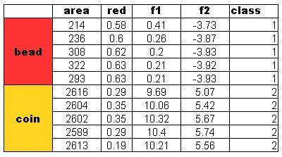
A perfect classification resulted from this method and with these features. I tried using the blue and green feature for classification also. Recall from Activity 14 that the green feature gives poor classification and blue gives a perfect classification. The results are:
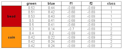
Also a perfect classification was obtained. However, when I tried to use the Red and Green feature, the same classification as that in Activity 14 was obtained. We can say that the red and green feature values of the beads and coins are near each other. Hence we cannot classify them perfectly using the said features. To compensate this, we can use a feature that is distinct for each class and combine it with the problematic feature. This is the technique I have used and it worked.

For this activity, I give myself a 10/10 for this activity for doing it alone and for being able to get a perfect classification.

CODE:
x=[214 0.58 0.54 0.45;
236 0.6 0.56 0.46;
308 0.62 0.56 0.49;
322 0.63 0.56 0.5;
293 0.63 0.56 0.5;
2616 0.29 0.24 0.13;
2604 0.35 0.31 0.14;
2602 0.35 0.31 0.14;
2589 0.29 0.25 0.13;
2613 0.19 0.18 0.09];

test = [247 0.57 0.52 0.44;
208 0.54 0.51 0.42;
192 0.55 0.53 0.43;
194 0.52 0.5 0.41;
193 0.52 0.5 0.41;
2736 0.33 0.3 0.14;
2835 0.43 0.4 0.2;
2904 0.47 0.42 0.22;
2925 0.47 0.42 0.24;
2874 0.45 0.42 0.24];


y=[ 1 1 1 1 1 2 2 2 2 2];
y=y';

x1=x(1:5,:);
x2=x(6:10,:);

mu1 = [sum(x1(:,1))/5 sum(x1(:,2))/5];
mu2 = [sum(x2(:,1))/5 sum(x2(:,2))/5];

mu = [sum(x(:,1))/10 sum(x(:,2))/10];

x1o=[x1(:,1)-mu(:,1) x1(:,2)-mu(:,2)];
x2o=[x2(:,1)-mu(:,1) x2(:,2)-mu(:,2)];

c1 = (x1o'*x1o)/5;
c2 = (x2o'*x2o)/5;

C=(c1*5 + c2*5)/10;
Cinv = inv(C);

p = [1/2; 1/2];

f1=[];
f2=[];

for i = 1:10;
xk = test(i, :);
f1(i) = mu1*C*xk' - 0.5*mu1*C*mu1' + log(p(1));
f2(i) = mu2*C*xk' - 0.5*mu2*C*mu2' + log(p(2));
end

class = f1 - f2;
class(class >= 0) = 1;
class(class < 0) = 2;

Reference:
[1] http://people.revoledu.com/kardi/tutorial/LDA/LDA.html

Activity 14: Pattern recognition

In this activity, we are to classify objects to classes using the Euclidian mean approximation. A training set is used to extract certain features present in all the classes and is distinct within each class. The mean feature of the training set is used to classify objects of unknown class. The objects I used for this activity are beads from a rosary and 25-centavo coins. These are shown below.

From this set of objects, 5 coins and 5 beads were used as a training set. To extract the features, I used parametric segmentation used in activity 12. The features extracted are the average red (R), green (G), and blue (B) color in the image. Also extracted was the area obtained from the segmented image by first inverting the image using GIMP and then binarizing it in Scilab. The resulting features and the mean features are shown in the table below.

The remaining 5 images of each class were used as the test set. The same processes were done to extract the features of test objects. Afterwhich, the features from each objects were subtracted from the mean feature obtained in the training set. Specifically,

where Dj is the distance of one feature of the test object x from the mean feature mj of each class.

An object is classified as the object in a class where Dj is minimum. The classification in this case was done in Excel. The results are as follows:
Note that 1 = bead and 2 = coin for the classification. From the tables, it can be readily seen that a 100% classification is obtained by examining the area and the blue color present in the images. For the green and red colors, poor classifcation was obtained. This is because the obtained red and green features from the test objects have almost nearvalues. We can conclude that classification by using the Euclidian mean is effective only to a certain extent.

I give myself an 8/10 for this activity for poor classification from the red and green colors and for doing the acivity alone. ^_^

Activity 12: Color Image Segmentation

For this activity, we are to select a region in the image with a particular color. First we have to transform the color space into a normalized chromaticity coordinates. To do this the following transformations are used:
Since 1=r+g+b, b=1-r-g. Therefore we can transform the color space (3-D) into two coordinate space (2-D), with the brightness associated with I. The image and patch used is shown below:

(Image taken from http://www.magicbob2000.com/resources/Cups%20&%20Balls%20Blue.jpg)

Patch

Two methods were used in this activity - parametric and nonparametric. For parametric a Gaussian Probability Distribution is used. The equation of which is given by
for the red values. The same is true for the green values (p(g)). The probability that a given pixel is inside the region of interest is dictated by prob=p(r)*p(g). For the nonparametric method, histogram backprojection is used. The pixel value in the histogram is used to backproject the value for a particular pixel. The histogram , result of parametric and nonparametric estimation of the image used is shown below:

Histogram

Parametric

Nonparametric

Although both estimations would suffice, a better segmentation is achieved with parametric estimation. It is also interesting that even the red "thingy" is well seen for parametric estimation. For the image used, the objects were separated from the background and from each other. Note however that we are only interested in segmenting the blue cups. Strictly speaking we did not segment the red "thingy". It just so happened that the background is violet (both with red and blue) which are the colors of the object that is why a gray color can be observed. Recall that when segmenting, what happens is that the region of interest becomes white. Any other color has different value.

Code:
stacksize(4e7);
chdir("C:\Documents and Settings\mimie\Desktop\186-12"); patch = imread("patch.jpg"); image = imread("cups.jpg"); ave = patch(:,:,1)+patch(:,:,2)+patch(:,:,3)+1e-7;
R = patch(:,:,1)./ave;
G = patch(:,:,2)./ave;
B = patch(:,:,3)./ave;

r = R*255;
g = G*255;

ave2 = image(:,:,1)+image(:,:,2)+image(:,:,3)+1e-7;
r2 = image(:,:,1)./ave2;
g2 = image(:,:,2)./ave2;
b2 = image(:,:,3)./ave2;
f = zeros(256,256);
for i=1:size(r,1)
for j=1:size(r,2)
x = abs(round(r(i,j)))+1;
y = abs(round(g(i,j)))+1;
f(x,y) = f(x,y)+1;
end
end
//imshow((frequency+0.0000000001));
//mesh(frequency);
//xset("colormap",jetcolormap(256));

\\\\parametric
rmean = mean(R);
rdev = stdev(R);
gmean = mean(G);
gdev = stdev(G);
rprob = (1/(rdev*sqrt(2*%pi)))*exp(-((r2-rmean).^2)/2*rdev);
gprob = (1/(gdev*sqrt(2*%pi)))*exp(-((g2-gmean).^2)/2*gdev);
prob = rprob.*gprob;
prob = prob/max(prob);
scf(0); imshow(image);
scf(1); imshow(prob,[]);

\\\\nonparametric
R2 = r2*255;
G2 = g2*255;
s = zeros(size(image,1),size(image,2));
for i = 1:size(R2,1)
for j = 1:size(R2,2)
x = abs(round(R2(i,j)))+1;
y = round(G2(i,j))+1;
s(i,j) = f(x,y);
end
end
scf(1); imshow(log(s+0.000000000001),[]);
scf(2); imshow(image);

Note:
Comment the parametric to use nonparametric


For this activity, I give myself an 8/10 since I'm not sure if I fully understand the activity.

Activity 11: Camera Processing

In this activity, we observed the effect of different white balancing options in cameras. Also, we applied the white patch and gray world algorithms on improperly white balanced images. Both RGB objects and objects with same color but different hues were used. It was found that for all images used, it is better to use the white patch algorithm.

For the first part, the same set of images were captured under different white balancing options in the camera. The white balancing options used were cloudy, daylight, fluorescent, fluorescentH, and tungsten. Capturing the images under these conditions is like illuminating the object with a light source with the same color temperature as the white balancing conditions. The images are shown below. The image captured under automatic white balancing is also included for comparison. Note that in the images the order is as follows

automatic white balanced
cloudy daylight fluorescent
fluorescentH tungsten

RGB

GREEN

From the images it can be observed that image taken under the tungsten condition is obviously improperly white balanced. The supposedly white paper appeared blue.

The white patch and gray world algorithms is then applied to these images to for white balancing. Each image has RGB values. In the white patch algorithm, we get a patch from the image that is supposedly white. The RGB value of this patch is used to divide the RGB value of the whole image such that Rn = R/Rw, Gn=G/Gw and Bn=B/Bw where Rn,Gn, Bn are the white balanced RGB values, R,G,B are the original RGB values and Rw,Gw,Bw are the RGB values of the patch.

For the gray world algorithm, it is assumed that the average color is gray. The key term here is "average". To operate the gray world algoirthm, we used average of the R,G, and B values and used this to divide the RGB values of the original image.

The following images are the result of the white patch and gray world algorithms on the images.

RGB IMAGES
Cloudy
Daylight
Fluorescent
FluorescentH
Tungsten

Notice that better images result from the white patch algorithm. The gray world algorithm produces a very bright image. This is maybe because white dominates in the image where it was applied.

GREEN IMAGES

Cloudy
Daylight
Fluorescent
FluorescentH
Tungsten

Like in the RGB images, the white patch algorithm obviously works better. Again, brighter images are observed in the gray world algorithm. Notice though that yellow green notebook became yellow when both algorithms were applied. This may be because the yellow color of the notebook is stronger than that of its green color.

The code:
stacksize(4e7)
rgbwp=imread("F:\186-11\wp.jpg");
rgb=imread("F:\186-11\green\tungsten.jpg");

rw=rgbwp(:,:,1);
gw=rgbwp(:,:,2);
bw=rgbwp(:,:,3);

r=rgb(:,:,1);
g=rgb(:,:,2);
b=rgb(:,:,3);

//white world
Rw = sum(rw)/(size(rgbwp,1)*size(rgbwp,2));
Gw = sum(gw)/(size(rgbwp,1)*size(rgbwp,2));
Bw = sum(bw)/(size(rgbwp,1)*size(rgbwp,2));


//gray world
Rg = mean(r);
Gg = mean(g);
Bg = mean(b);


rr=r/Rw;
rg=g/Gw;
rb=b/Bw;

gr=r/Rg;
gg=g/Gg;
gb=b/Bg;

chuva = [];
chuva(:,:,1)=rr;
chuva(:,:,2)=rg;
chuva(:,:,3)=rb;
chuva(chuva>1) = 1;
//scf(0), imshow(chuva);
//scf(1), imshow(rgb);

chuva2 = [];
chuva2(:,:,1)=gr;
chuva2(:,:,2)=gg;
chuva2(:,:,3)=gb;
chuva2(chuva2>1) = 1; //pin values to 1
//scf(1), imshow(chuva2);

imwrite(chuva,"F:\186-11\result\green\tungstenw.jpg");
imwrite(chuva2,"F:\186-11\result\green\tungsteng.jpg");

Notice that the image values are all pinned to 1.

For this activity, I give myself a 10/10 since I believe I was able to perform the task asked for this activity. Thank you to Neil and Earl for the discussion we had.